The following is a record of my final project for Math888 Fall 2022.
Defining the Problem
Consider an agent interacting with a Markov Decision Process (MDP) with state space \(S\), action space \(A\), rewards \(R\), and transition probabilities \(P\). At each time point \(t\), the agent observes a state \(s_t\in S\), chooses an action \(a_t\in A\) based on their policy \(\pi_t\), transitions to a new state \(s_{t+1}\) given by transition probability \(p(s_{t+1}\|s_t,a_t)\) unknown to them, and receives a reward \(r_t(s_{t}, a_{t})\) from the environment. The agent is given a goal like “reach 40 points in less than 20 moves.” Let \(M_i\) be the \(i\)-th MDP an agent interacts with. Let \(T\) be the number of MDPs an agent interacts with.
I want to know if we can give the agent a sequence of MDP problems to reduce biases in the agent’s approach to the problems. Biases in executive function decrease flexibility in problem solving by restricting the space of possible policies and/or increasing the time it takes to arrive at some policies, so if we can decrease an agent’s biases we could potentially train them to solve problems more quickly and more accurately.
We define \(Y_T\) to be the number of optimal choices the agent makes while interacting with \(M_T\). Note that optimality could be defined in terms of the underlying MDP or in terms of the experience of the agent, so \(Y_T\) can depend on both the MDP and the agent. We can define a function \(Y_T(M_1,M_2,\dots,M_T)\) that maps the history of MDPs an agent interacts with to the number of optimal choices they make while interacting with \(M_T\).
We are then interested in evaluating the conditional average causal excursion effect \(\mathbb{E}[Y_T(M_1, M_2, \dots, m_T) - Y_T(M_1, M_2, \dots, m_T')]\).
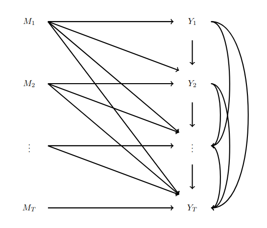
Note that \(Y_T\) depends on the entire history of the MDPs and prior actions.
Identification
Note: \(Y_{i}(m_{\leq j}) := Y_i(m_1,\dots,m_j)\).
We intervene on each MDP independently, leading to the following SWIG:
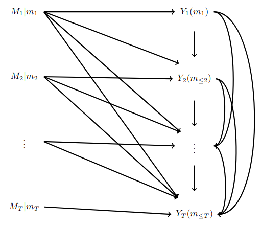
This allows us to conclude that \(M_i\perp \!\!\! \perp Y_j(m_{\leq j})\), and more importantly, \(M_i\perp \!\!\! \perp Y_j(M_{\leq j-1}, m_j)\) for any \(i,j\in[T]\).
For \(i\in[T]\), we need a positivity assumption that \(P(M_i=m_i)>0\) and \(P(M_i=m_i')>0\), a consistency assumption that \(Y_i(M_{\leq i}) = Y_i\), and the standard SUTVA assumption that the mapping \((m_{\leq i}) \mapsto Y_i(m_{\leq i})\) is well defined.
We therefore get via linearity
\[\mathbb{E}[Y_T(M_{\leq T-1}, m_T) - Y_T(M_{\leq T-1}, m_T')] = \mathbb{E}[Y_T(M_{\leq T-1}, m_T)] - \mathbb{E}[Y_T(M_{\leq T-1}, m_T')].\]Then, since \(M_T\perp \!\!\! \perp Y_T(M_{\leq T-1}, m_T)\) and \(M_T\perp \!\!\! \perp Y_T(M_{\leq T-1}, m_T')\) we get
\[= \mathbb{E}[Y_T(M_{\leq T-1}, m_T) \mid M_T=m_t] - \mathbb{E}[Y_T(M_{\leq T-1}, m_T') \mid M_T=m_t'] .\]Note these conditionals are well defined via our positivity assumption. This conditioning gives us
\[= \mathbb{E}[Y_T(M_{\leq T}) \mid M_T=m_t] - \mathbb{E}[Y_T(M_{\leq T}) \mid M_T=m_t'].\]So by consistency we arrive at
\[= \mathbb{E}[Y_T \mid M_T=m_t] - \mathbb{E}[Y_T \mid M_T=m_t']\]which is a statistical estimand we can estimate using the data.
Notice that the number of possibilities for the history, which will impact \(Y_T\), increases very quickly, so there are many estimates we would need to compute to draw conclusions from. However, the estimand at the end does not explicitly rely on the history.
The Data
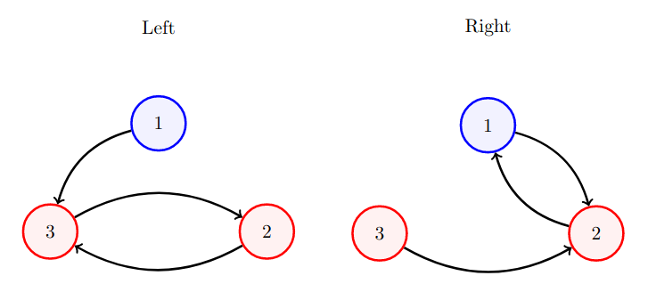
In the Seqer dataset, if we consider just the first MDP played by each participant the MDPs all have 3 states, the transitions were deterministic, and the actions were binary. Rewards depended only on the next state. Two states each had reward probability 0.2, while the other state had reward probability 0.8. The high-reward state and one low-reward state had the same optimal action (both left or both right), while the other state transitioned the same way independent of action. I will call a state definite if it has an optimal action and indefinite if transition is independent of action. Note that an optimal action in a definite state leads to a transition to the other definite state. This leads to twelve different MDPs, because there are 3 options for high reward state, 2 options for optimal action, and 2 options for the indefinite state. Each participant completed 20 actions, and at each time step saw a diagram of which state they were in.
For example, Type 0, shown below, has high-reward state 1 (shown in blue), optimal action of right, and indefinite state 3 which is counterclockwise from the high reward state. Note that you can determine the indefinite state by determining which state allows for a 1-step return to the high-reward state.
Let \(a_{ji}\) be the \(i\)-th action chosen by participant \(j\), and \(s_{ji}\) be the \(i\)-th state shown to participant \(j\). I defined an optimality function \(f(a_{ji},s_{ji})=1_{a_{ji}\text{ was optimal for state }s_{ji}} + .5\cdot{1_{s_{ji} \text{ is indefinite}}}\) and took \(Y_j - \frac{1}{10} \sum_{i=1}^{10} f(a_{ji}, s_{ji})\). This gives a value between 0 and 1, where higher values mean more optimal choices were made. Note that I am only considering the last 10 choices, assuming that the first 10 will be mostly random as people explore the problem.
Outcome Regression
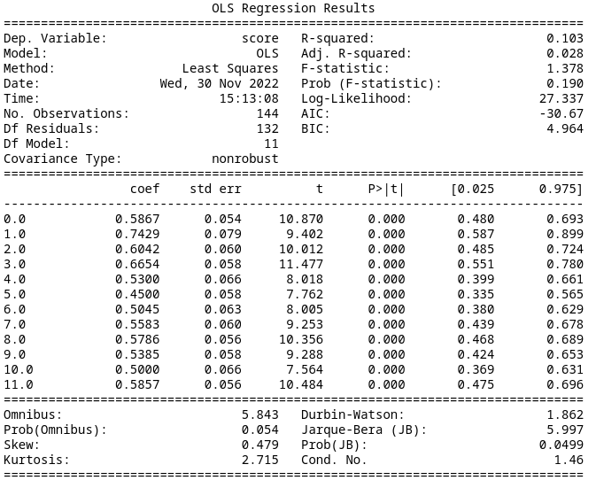
If we encode the MDP type using a one-hot encoding (for MDP type \(k\) we form a vector with 1 in the \(k\)-th position and 0 everywhere else), we can then perform outcome regression. I used an ordinary least squares linear model from the Python package statsmodels. In the end I implemented 7 models and then used the Akaike Information Criterion (AIC) to assess model fit. Note that AIC values are relative, with lower being better, and lower by >2 is significantly better.
We have between 7 and 15 trials of each MDP type. As a result, I tried grouping the data based on the three characteristics identified previously to overcome some of the instability that occurs with such small sample sizes.
Model 0
Treating each of the 12 MDP types separately results in an AIC of -30.67. The summary data is below.
Model 1
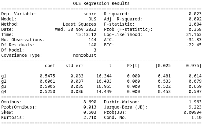
If we assume that participants recognized that the orientation of the diagram was irrelevant so we can reorder the states to remove the stratification by placement of the high reward state, we can group the MDP types into 4 groups of 3. Fitting a linear regression in the same manner as before results in an AIC of -34.33. This is better than the prior model. The summary data is below.
Model 2
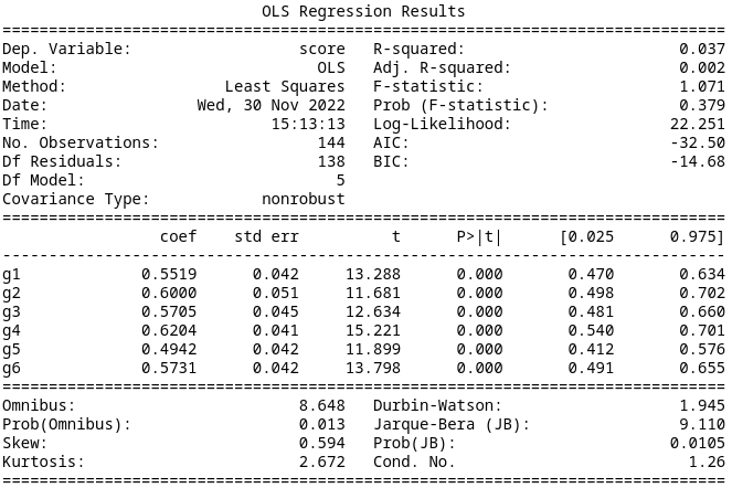
If we assume participants are not affected by which action is optimal, we get six pairs of MDPs. This results in an AIC of -32.50. Therefore Model 1 is better but only slightly. The summary data is below.
Model 3
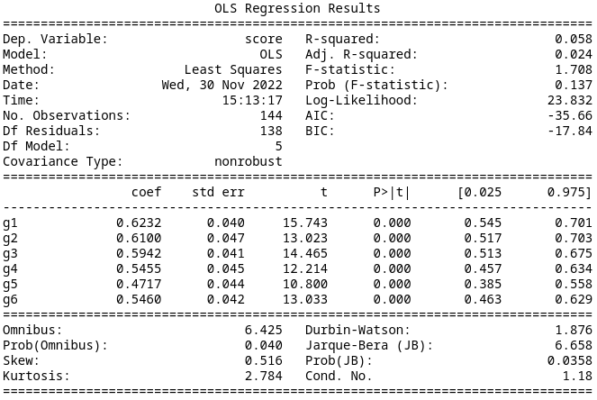
If we assume that the position of the indefinite state is irrelevant, we again arrive at six pairs of MDPs. This gives an AIC of -35.66, so this is better than Model 0 and Model 2, but on par with Model 1. The summary data is below.
Model 4
Further reducing the categories by assuming that only the optimal action is relevant gives an AIC of -35.03, which is again better than Model 2, but comparable with Model 1 and Model 3. The summary data is below.

Model 5
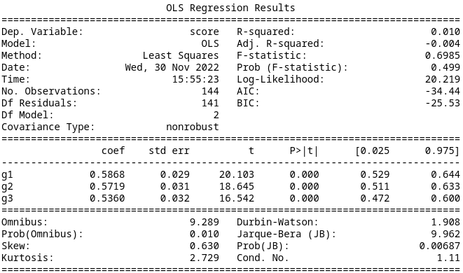
If we instead pay attention only to the location of the high reward state, we find an AIC of -34.44. This is comparable to the previous models. The summary data is below.
Model 6
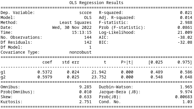
Finally, if we consider just the location of the indefinite state relative to the high-reward state, we get an AIC of -38.02. This is the lowest AIC, and is a large improvement. The summary data is below.
Results
Since we have a randomized control trial, and only look at the first MDP, identification is a straight forward application of the usual assumptions. With the linear regression model, it amounts to taking the difference of the coefficients of the group \(m_j\) belongs to and the group \(m_j'\) belongs to. Using Model 6 since it was the best, we arrive at \(0.5372-0.5979=-0.0607\) where for MDPs in Group 1 the indefinite state is counterclockwise from the high-reward state and for MDPs in Group 2 the indefinite state is clockwise from the high-reward state.
This seems to suggest that performance is better when the indefinite state is clockwise from the high-reward state, and this characterizes the difference between MDPs.
Sensitivity
One strength of this experimental design is that because the MDPs were randomly designed, we do not have to worry about unmeasured confounding. However, we still have the SUTVA and consistency assumptions that are untestable.
The major assumptions I made were in the groupings I considered for the models. Since the data is categorical, Model 0 is fully saturated so I have a baseline model that does not assume linearity in any of the parameters. However, the six other models I evaluated assume that MDPs within each group can be treated interchangeably. They are also not the only possible groupings, but the number of possible groupings makes testing them all impractical.
The other major assumption I made was that people finished the exploratory part of their problem solving by the last 10 steps. One way of seeing if that is true, is to repeat the same analysis using the data from when half of the participants played their first MDP over again. This is the resulting analysis:
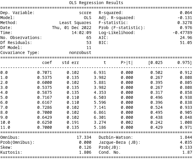
Model 0
Treating each of the 12 MDP types separately results in an AIC of 24.96. The summary data is below.
Model 1
If we assume that participants recognized that the orientation of the diagram was irrelevant so we can reorder the states to remove the stratification by placement of the high reward state, we can group the MDP types into 4 groups of 3. Fitting a linear regression in the same manner as before results in an AIC of 12.52. This is significantly better than the prior model. The summary data is below.
Model 2
If we assume participants are not affected by which action is optimal, we get six pairs of MDPs. This results in an AIC of 15.01. The summary data is below.
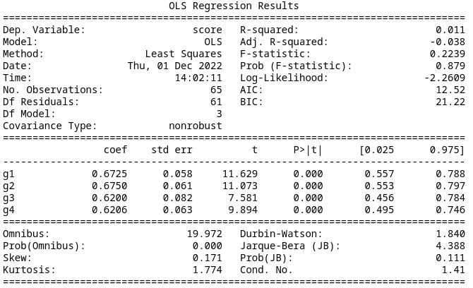
Model 3
If we assume that the position of the indefinite state is irrelevant, we again arrive at six pairs of MDPs. This gives an AIC of 16.44. The summary data is below.

Model 4
Further reducing the categories by assuming that only the optimal action is relevant gives an AIC of 9.223, which is significantly better than Model 1. The summary data is below.

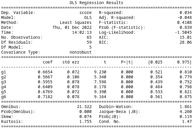
Model 5
If we instead pay attention only to the location of the high reward state, we find an AIC of 11.19. This is slightly worse than the previous model. The summary data is below.
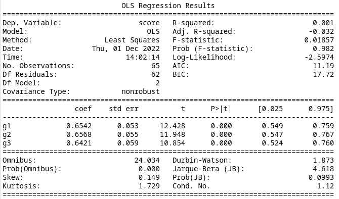
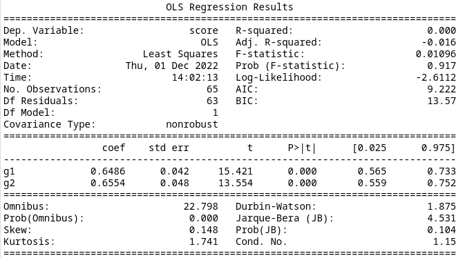
Model 6
Finally, if we consider just the location of the indefinite state relative to the high-reward state, we get an AIC of 9.222. This is the lowest AIC, but is not a significant improvement. The summary data is below.
Results
This complicates the interpretation of the prior results. Here Model 4 and Model 6 are a little better than Model 5, but neither is clearly better than the other. It seems that grouping based on any of the three characteristics individually leads to a better model than combining them.
Conclusion
I started a preliminary analysis of the Seqer dataset, to see what characteristics of basic MDPs impact people’s ability to solve them for the optimal decisions. It seems like the relative positioning of the high reward state and the least rewarding state has more of an impact than I expected, but the data is very noisy so I cannot say that with any surety. I also did not get to analyzing anything past the first MDP. In the future, I would like to try different groupings or parameters of the MDPs. Eventually this will contribute to our understanding of how humans learn and make decisions under uncertainty.